Overview
Functional connectivity can be a powerful approach to studying the brain, but must be used
carefully. Numerous artifacts can affect the quality of your results. Our approach is to
first preprocess fMRI data using FMRIPREP to quantify head motion and other confounds,
then to use these estimates in xcpEngine to denoise the fMRI signal and estimate
functional connectivity.
To process your data from scanner to analysis, the steps are generally
Steps 1 and 2 are well-documented and have active developers who can help you through these steps;
this documentation will help you get started with step 3 (xcpEngine).
Installation
The easiest way to use xcpEngine on your laptop or personal computer is to install Docker and
the xcpEngine python wrapper. Ensure that Docker has access to at least 8GB of memory.
If you are on an HPC system where you cannot run Docker, you can use Singularity. Be sure one
of these is installed and then install the xcpEngine container wrapper using Python:
Then install the wrapper using:
pip install xcpengine-container
Once this completes you can run xcpEngine without explicitly running Docker:
xcpengine-docker \
  -d /xcpEngine/designs/fc-36p.dsn \
  -c /path/to/cohort.csv \
  -r /path/to/data/directory \
  -i /path/to/workingdir \
  -o /path/to/outputdir
or Singularity:
xcpengine-singularity \
  --image /path/to/xcpEngine.simg \
  -d /xcpEngine/designs/fc-36p.dsn \
  -c /path/to/cohort.csv \
  -r /path/to/data/directory \
  -i /path/to/workingdir \
  -o /path/to/outputdir
Continue reading to learn about the arguments and be sure to use the correct executable
xcpengine-singularityfor Singularityxcpengine-dockerfor Docker
Getting started
Once your data is processed by FMRIPREP you are ready to use xcpEngine. FMRIPREP
can write preprocessed data out in multiple spaces. At the moment, xcpEngine only supports
volume data, meaning that T1w and MNI152NLin2009cAsym are the only usable options
for FMRIPREP’s --output-spaces flag. Either is a viable starting point. Choosing
MNI152NLin2009cAsym is the most straightforward route, but T1w adds the possibility
of using a custom template for normalization. Here we’ll assume you want to process data that
has already been resampled in MNI space (i.e. --output-spaces MNI152NLin2009cAsym was
part of your FMRIPREP call) and you’re running on your laptop with Docker installed.
Step 1: Create a cohort file
xcpEngine reads images and metadata from a user-provided csv file called a Pipeline cohort file.
Briefly, the cohort file should contain
subject metadata (without special shell characters) in id columns and paths to images
written by FMRIPREP in the img column. In this example use case, the cohort file
might be saved as /home/me/cohort.csv and contain:
id0,img
sub-01,sub-01/func/sub-01_task-mixedgamblestask_run-01_space-MNI152NLin2009cAsym_desc-preproc_bold.nii.gz
We recommend making the paths relative to the --output-dir you used for FMRIPREP.
Step 2: Choose/Configure a Pipeline design
Not all functional connectivity pipelines are equally effective at addressing systematic noise
and artifacts. Many papers have proposed different denoising strategies, which may vary in
effectiveness. xcpEngine has many of the top performing de-noising strategies implemented
available as Pipeline design file that can specify the processing stages and calculation of output
measures.
A library of pipelines comes pre-packaged with xcpEngine and are
described in the accompanying paper. We test these design files before distributing xcpengine
and recommend using them as-is. Changes may produce poor-quality results.
These are pre-packaged in the images in /xcpEngine/designs and a full list
can be found in the GitHub repository (https://github.com/PennBBL/xcpEngine/tree/master/designs).
These designs implement the processing pipelines found in the following table:
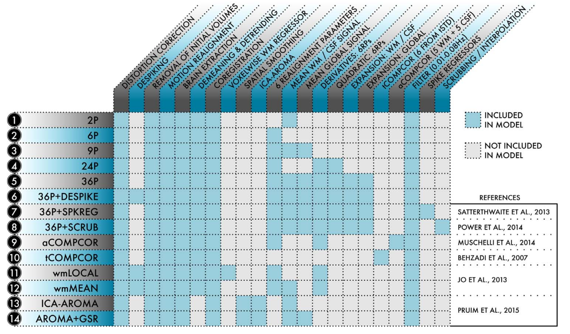
Available pipeline designs
Note
The poor-performance pipelines are not included. Also, you will need to adjust the thresholds for rmss for your TR (Temporal Censoring) if you’re using a pre-packaged design file.
Step 3: Process your data
To run your pipeline with Docker simply:
xcpengine-docker \
  -c /home/me/cohort.csv \
  -d /xcpEngine/designs/fc-36p.dsn \
  -i /home/me/work \
  -o /home/me/xcpOutput \
  -r /home/me/fmriprep_outputdir/fmriprep
Very similarly, the command for Singularity is:
xcpengine-singularity \
  --image /home/me/xcpEngine-latest.simg \
  -c /home/me/cohort.csv \
  -d /xcpEngine/designs/fc-36p.dsn \
  -i /home/me/work \
  -o /home/me/xcpOutput \
  -r /home/me/fmriprep_outputdir/fmriprep
Your outputs will be located on your computer in /home/me/xcpOutput and are ready for testing
hypotheses!